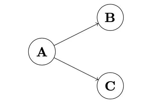
Here, I’ll walk through how to code causal modeling diagrams in TikZ, like the following:
TikZ is a package for LaTeX that is included in the base distribution. If you’re not sure what LaTeX is, or would like some help installing and getting started with it, I recommend AJ Hildrebrand’s site. Once you’re set up and have some familiarity with typesetting basic mathematical and logical formulas, then it’s time for TikZ!
Basic Stuff
The first thing to do is load TikZ in your preamble. We’ll also need to direct your compiler to load the following TikZ libraries: patterns, shapes, and decorations:
\usepackage
\usetikzlibrary
Next, let’s draw some basic shapes, for instance, a circle:
\begin{tikzpicture}
\draw[-] (0,0) circle (1cm);
\end{tikzpicture}
The \draw command tells us to draw something. We specify that what we want is a solid line (that’s the [-] part). Next, we have the coordinates specifying the center of the circle, that’s (0,0). We specify the radius of the circle as 1cm. Finally, notice that we end the command with a semicolon, ;. Note that TikZ is built on a grid system. We can overlay the grid to see what’s going on in the background:
\begin{tikzpicture}
\draw[help lines] (-2,-2) grid (2,2);
\draw[-] (0,0) circle (1cm);
\end{tikzpicture}
We also use the \draw command to draw lines and arrows:
\begin{tikzpicture}
\draw[help lines] (-2,-2) grid (2,2);
\draw[-] (0,0) circle (1cm);
\draw[-] (-2,-2) -- (0,0);
\draw[->] (-1,1.5) -- (1.5,1.5) -- (1.5,-1.5);
\end{tikzpicture}
The other crucial component of TikZ is the \node command, which allows you to specify a point with various properties, like a circle that contains some text:
\begin{tikzpicture}
\node[circle,draw] at (0,0) (A) ;
\end{tikzpicture}
Here, draw specifies that we want to draw the circle around the node, at (0,0) tells us where the node is located on the grid, (A) labels the node (this will be useful for referring back to it later), and {A} specifies what is to be written inside of the node. We can position nodes relative to one another using the commands
right of
left of
above of
below of
in various combinations:
\begin{tikzpicture}
\node[circle,draw] at (0,0) (A) ;
\node[circle,draw,right of=A] (B) ;
\node[circle,draw,below right of=B] (C) ;
\end{tikzpicture}
Finally, we can offset nodes from their relative positions using the xshift and yshift commands:
\begin{tikzpicture}
\node[circle,draw] at (0,0) (A) ;
\node[circle,draw,right of=A] (B) ;
\node[circle,draw,below right of=B,xshift=1cm] (C) ;
\node[circle,draw,below right of=B,yshift=-1cm] (D) ;
\end{tikzpicture}
Putting Things Together
We can now start to combine nodes and arrows to generate basic causal model diagrams. To start, I’ll start our tikzpicture with the command \begin{tikzpicture}[node distance=2cm], which will specify that we want 2cm between nodes rather than the usual 1cm. Let’s start simple:
\begin{tikzpicture}[node distance=2cm]
\node[circle,draw] at (0,0) (A) {\bf A};
\node[circle,draw,right of=A,yshift=1cm] (B) {\bf B};
\node[circle,draw,right of=A,yshift=-1cm] (C) {\bf C};
\draw[->] (A) -- (B);
\draw[->] (A) -- (C);
\end{tikzpicture}
To draw the lines connecting B and C to D, notice that I specify the path more explicitly, marking the waypoints I want the line to trace through:
\begin{tikzpicture}[node distance=2cm]
\node[circle,draw] at (0,0) (A) {\bf A};
\node[circle,draw,right of=A,yshift=1cm] (B) {\bf B};
\node[circle,draw,right of=A,yshift=-1cm] (C) {\bf C};
\node[circle,draw,right of=B,yshift=-1cm] (D) {\bf D};
\draw[->] (A) -- (B);
\draw[->] (A) -- (C);
\draw[->] (B) -- (3,1) -- (3,0) -- (D);
\draw[-] (C) -- (3,-1) -- (3,0);
\end{tikzpicture}
We can add squiggly lines, label nodes, and make them either bold or dashed or dotted using the commands:
\draw[snake]
\node[thick]
\node[dashed]
\node[dotted]
\node[label=above: … ]
\begin{tikzpicture}[node distance=2cm]
\node[circle,draw,dashed] at (0,0) (A) {\bf A};
\node[circle,draw,right of=A,yshift=1cm,dotted] (B) {\bf B};
\node[circle,draw,right of=A,yshift=-1cm,thick,label=above:\tiny{\sf F}] (C) {\bf C};
\draw[->] (A) -- (B);
\draw[->] (A) -- (C);
\draw[snake] (-1,2) -- node[at start, above]  (-1,-2);
\end{tikzpicture}
Some Finishing Touches
You’re now on your way to making some fun causal modeling diagrams. I want to conclude with a few advanced features to get things looking even better.
The first is a tikzset, which you can use to define global properties that you can call on inside of your tikzpictures. You’ll want to add tikzsets to your preamble (before \begin{document}). Here is one:
\tikzset{
intervention/.style ={node distance=2cm},
p/.style={circle,draw,minimum size=0.5cm},
arrow/.style={->,>=stealth,shorten >=1pt},
snake/.style={-,decorate, decoration=snake}
}
What this does is specify my node distance and then defines three parameters: p, arrow, and snake. For instance, p/.style={circle,draw,minimum size=0.5cm} just allows me to write:
\node[p]
instead of
\node[circle,draw,minimum size=0.5cm]
Now, our code above can be simplified to:
\begin{tikzpicture}[intervention]
\node[p] at (0,0) (A) {\bf A};
\node[p,right of=A,yshift=1cm] (B) {\bf B};
\node[p,right of=A,yshift=-1cm] (C) {\bf C};
\node[p,right of=B,yshift=-1cm] (D) {\bf D};
\draw[arrow] (A) -- (B);
\draw[arrow] (A) -- (C);
\draw[arrow] (B) -- (3,1) -- (3,0) -- (D);
\draw[-] (C) -- (3,-1) -- (3,0);
\end{tikzpicture}
(Notice also the nicer arrowheads and the spacing on the arrows is a bit cleaner too!)
Finally, we can add split nodes using the circle split command in \node to create:
\begin{tikzpicture}
\node[circle split, draw] (A) {{\bf A} \nodepart {\bf B}};
\end{tikzpicture}
There you have it! Hopefully this gives you a sense of how to make your own causal modeling diagrams in TikZ. Check back in for more tutorials like this soon.


